
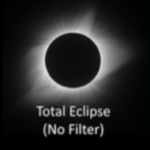
 What Is a Total Solar Eclipse? A total solar eclipse occurs when the moon passes between the sun and the Earth, causing the moon to completely block the face of the sun. This period of total eclipse is referred to as “totality.” Indiana is in the path of totality and will experience a [...]
 Free dental screenings will be held on Friday, February 2nd from 10:30am- 3pm. Please click on the link below for more information! Give Kids a Smile Flyer 2024
 Immunizations and other services are available by appointment through the Nurse of the Day program at the Marion County Public Health Departments. Click here for information about District Heath Office locations, hours and phone numbers to call for an appointment. Immunizations for children and young adults from birth through age 26 are also available at [...]
 Birth Certificate – English/Spanish Please click here to visit the Vital Records webpage.
Health and Hospital Corporation of Marion County’s Division of Public Health is known as the Marion County Public Health Department (MCPHD). MCPHD has served the residents and visitors of Marion County, Indiana for nearly 100 years. The area that MCPHD covers includes the City of Indianapolis, Beech Grove, Lawrence, Speedway, and Southport. The mission of the department is to promote physical, mental, and environmental health, prevent and protect against disease, injury, and disability. The health department operates two service bureaus: the Bureau of Environmental Health (BEH), the Bureau of Population Health (BPH) and Public Health Administration. It is enabled through Indiana Code 16-22-8.
